Guy Fipps and Frank J. Dainello
Most growers recognize that agriculture is a very risky business. Irrigation is a means of reducing some of the risk in agriculture, and is necessary for vegetable production in many areas of the State. The hope is that additional revenue from improved quality and yields will not only pay for the costs of purchasing and operating the irrigation system, but also will result in greater profits. Choose the correct system for your particular situation. Consider carefully the first costs of buying and installing the system, as well as the continuing costs for pumping, operation, labor and maintenance.
Good management practices also are very important. Correct irrigation timing and amount of water often make the difference between profit and loss in an irrigation operation. Additionally, the use of pressure gauges and flow meters to monitor irrigation system performance allows for timely detection of problems. This chapter will cover some of the basic factors that should be considered in selection and management of irrigation systems for vegetable production in Texas. Space limitations prevent detailed discussion of all the aspects of irrigation. Additional references and sources of information are provided for each topic.
Irrigation System Selection
There are many types of irrigation systems on the market that are suitable for vegetable production. Systems vary greatly in costs and have different operation and site requirements. Many factors determine which system is right for you. Some of the factors to consider and data needed for a proper irrigation system design are listed in Table V-1. Contact your local office of the USDA Soil Conservation Service (SCS), irrigation dealer or county extension agent for assistance in completing a site evaluation. The booklet “Planning for an Irrigation System” (Reference 1) contains a complete discussion of the factors to consider and types of systems. Another good source of information for general planning purposes is the “Soil Survey” by the USDA Soil Conservation Service (SCS) for your county and specific site. It provides general recommendations on the suitability of soil types for the irrigation of specific crops.
Table V-1. Principal Data Needed for Farm Irrigation System Design
| Data | Specific Requirements |
|---|---|
| Crop | Distribution and area of each crop to be grown; Suitability of each crop to climate, soils, farming practices, markets; Planting dates for each crop to be grown over the expected life of the project |
| Soil | Area distribution of soils, Water holding and infiltration characteristics, Depth, Drainage requirements, Salinity, Erosion potential of each soil |
| Water Requirement | Data for estimating daily and seasonal water requirements for each crop |
| Water Supply | Location of water source, Amount of water or pumping capacity, water surface elevation; Hydrologic and water quality information for assessing the availability, costs, and suitability of the water for irrigation; Water rights information |
| Energy Source | Location, availability, and type of source(s); Cost information |
| Capital and Labor | Capital available for system development, Level of technical skill, Cost of labor |
| Other | Topographic map showing location of roads, buildings, drainways, and other physical features that influence design, financial situation of farmer, or farmer preferences |
Critical Factors to Consider
- Water Supply: The amount of water available and the cost of the water (due to pumping or direct purchase) will determine the amount of land that can be irrigated and often the type of system you should use. Depending on location, climate, type of crop and irrigation system efficiency, a water supply (well yield or delivery rate) from 3 to 15 gallons per minute (GPM) is required for each acre to be irrigated. If the supply of water is limited or very expensive, then consider only the most efficient types of systems (Table V-2).
Table V-2. Typical Overall On-farm Efficiencies for Various Types of Irrigation Systems (adapted from James, 1988)
| System | Overall Efficiency (%) |
|---|---|
| Surface a) Average b) Land leveling and delivery pipeline meeting design standards c) Tail water recovery with (b) d) Combination level and graded flow irrigation (max 0.1% grade and block ends) e) Surge |
50 – 80 50 70 80 80 – 95 60 – 90 |
| Sprinkler | 55 – 75 |
| Center Pivot | 55 – 75 |
| LEPA a) Bubble Mode b) Spray Mode |
95 – 98 80 – 85 |
| Drip | 80 – 90 |
* Surge has been found to increase efficiencies 8 to 28% over nonsurge furrow systems.
** Trickle systems are typically designed at 90% efficiency, short laterals (< 100 ft) or systems with pressure compensating emitters may have higher efficiencies
- Water Quality: Is the water suitable? Be sure to have a water sample analyzed. The Soil and Water Testing Lab at Texas A&M University will provide recommendations on the suitability of your water for irrigation of specific crops. Contact your county extension agent for forms and information. Also, water high in salts may cause foliar damage if sprayed directly on the plants. In these cases consider systems that deliver water directly on or below the surface such as drip, surface or LEPA systems. Special consideration is also needed in the placement of drip tubing and emitters when irrigating with saline water.
- Soil Type: Light sandy soils are not well suited to furrow or surface irrigation systems. Lateral water movement is restricted in these soil types. These soils are best irrigated by sprinkler or drip irrigation systems.
- Field Shape and Topography: Odd shaped field not easily irrigated with certain types of sprinkler systems such as center pivots. Rolling topography prohibits the use of furrow or surface systems because water cannot run up hill.
- Labor: Labor availability and costs are prime considerations. The labor and skill required for operation and maintenance varies greatly between systems. For example, studies have shown that about one-man-hour per acre is required for a hand-move sprinkler system. Mechanical move systems require 1/10 to ½ as much labor. Automated systems are more expensive to purchase, but may be more profitable when the labor costs over the life of the system are considered.
- Suitability: Choose a system that is compatible with your farming operations, equipment, field conditions and crops and/or crop rotation plan.
- Personal Preference: Select a system that you can live with. If you do not like your system, chances are you will not operate or maintain it properly.
Types of Systems
Irrigation systems may be grouped into three general types: surface, sprinkler and drip. Aspects of these systems are compared in Table V-3. Only a brief description of each type will be given here. For more information refer to Reference 1 and the other references at the end of this chapter. Other good sources of information are the County Extension Agent, the area SCS office and the local irrigation dealer.
Table V-3. Comparison of Irrigation Systems in Relation to Site and Situation Factors
| Site and Situation Factors | Well-Designed Surface Systems | Level Basins | Intermittent* Mechanical Move |
Continuous** Mechanical Move |
Solid Set and Permanent | Emitters and Drip Tubing |
|---|---|---|---|---|---|---|
| Infiltration Rate | Moderate to low | Moderate | All | Medium to high | All | All |
| Topography | Moderate slopes | Small slopes | Level to rolling | Level to rolling | Level to rolling | All |
| Crops | All | All | Generally shorter crops | All but trees and vineyards | All | High value required |
| Water Supply | Large streams | Very large streams | Small streams nearly continuous | Small streams nearly continuous | Small streams | Small streams continuous and clean |
| Labor Requirement | High, training required | Low, some training | Moderate, some training | Low, some training | Low to seasonal high, little training | Low to high, some training |
| Capital Requirement | Low to moderate | Moderate | Moderate | Moderate | High | High |
| Energy Requirement | Low | Low | Moderate to high | Moderate to high | Moderate | Low to moderate |
| Management Skill | High | Moderate | Moderate | Moderate | Moderate | High |
| Windy Conditions | Good | Good | Poor | Poor to excellent*** | Fair | Fair to excellent |
* Side roll, big guns, etc.
** Center pivot
*** Depends on type of water applicators
Adapted from: G.O. Schwab, R.K. Frevert, T.W. Edminster, and K.K. Barnes, Soil and Water Conservation Engineering, 1981. John Wiley & Sons, Inc., New York, pp 430-431.
Surface
Surface irrigation uses gravity flow to spread water over a field. A good supply of water (stream size) in GPM (gallons per minute) is needed. Surface systems are the least expensive to install, but have high labor requirements for operation. Skilled irrigators also are needed in order to obtain good efficiencies. Even if properly designed, surface systems tend to have low water application efficiencies. Low efficiencies result in higher pumping (or water costs) due to the increased amounts of water required. The SCS has developed the design standards used for surface irrigation and will design assistance.
The two most common surface systems used for irrigating vegetables in Texas are level basin and furrow systems.
Level basin (or dead level irrigation): With this method, water is applied over a short period of time to a completely level area enclosed by dikes or borders. The floor of the basin may be flat, ridged or shaped into beds. Basin irrigation is the most effective on uniform soils precisely leveled when large stream sizes (in GPM) relative to basin area are available. If properly designed and operated, level basin systems can attain high water application efficiencies.
Furrows are small, evenly spaced, shallow channels formed in the soil. Optimal furrow lengths are primarily controlled by the soil intake rate, furrow slope, set time and stream size. For most applications the stream size should be as large as possible without causing erosion. SCS has developed recommendations on maximum row length for specific soils and slopes. The major limitation of this system is the inability to apply small amounts of water at frequent intervals as needed by shallow rooted vegetable crops.
Combination level and graded flow irrigation systems are used in the Lower Rio Grande Valley. They have a maximum slope of 0.1 ft per 100 ft (0.1%) and block ends. With proper stream size, these systems can have good water application efficiencies.
Advantages of surface systems are: water deficits can be overcome rapidly; least expensive of the major types of irrigations systems; low maintenance, and usually require the lowest level of management.
Disadvantages of surface systems are: process the least water use efficiency; lack uniformity in water distribution, increase disease incidence especially in vining crops, and, periodic depletion of soil oxygen which can cause yield reduction.
For furrow irrigation, you should consider the following:
- Precision Land Leveling: improves water application efficiency. Leveling land is cost effective on many sites, and will pay for itself by increasing yields and reducing water losses.
- Gated Pipe: can result in a 35% to 60% reduction in water and labor costs. Gated pipe provides a more equal distribution of water into each furrow and eliminates seepage and evaporative losses which occur in unlined irrigation ditches. Gated pipe is available as the traditional aluminum pipe, the less expensive low head PVC pipe, the inexpensive “lay flat” plastic tubing. The lay flat tubing will last 3 to 5 seasons.
- Surge Flow Irrigation: is a variation on continuous flow furrow irrigation. Water usually is applied in cycles of one to three hours of alternating on/off periods. Surge works by taking advantage of the natural surface sealing properties of many soils. Surge often results in increased irrigation efficiencies and gives the grower the ability to apply smaller amounts of water at more frequent intervals. The automatic surge valves also are appealing because of reduction in labor. Researchers have found that for the clay silt soils found on the Texas High Plains, surge requires a stream size of 12 to 16 GPM for each furrow. Some experts claim that generally a stream size from 20 to 25 GPM is necessary. For more information on surge see Texas AgriLife Extension Publication L-2220 “Surge Flow Irrigation” (Reference 3.)
Sprinkler
Sprinkler irrigation is defined as a pressurized system where water is distributed through a network of pipe lines to and in the field and applied through selected sprinkler heads or water applicators. Sprinkler systems are more expensive than surface systems, but offer much more flexibility and control. They are suitable for most soil and topographic conditions, and can also be used for cooling and frost/freeze protection.
The basic components of sprinkler systems are illustrated in Figure V-1 and include a water source, a pump to pressurize the water, a pipe network to distribute the water through the field, sprinklers to spray the water over the ground, valves to control the flow of water, and flow meters and pressure gauges to monitor system performance. Many sprinkler systems also are very good for chemigation. There are many types of sprinkler devices available (only a few of the more common types of sprinkler systems are discussed here.) For more information see References 1, 2, 4, 5 and 9.
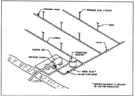
Figure V-1. Components of a typical sprinkler irrigation system. A flow meter and several pressure guages are used to monitor system performance.
Hand-Move and Portable Sprinklers: These systems employ a lateral pipeline with sprinklers installed at regular intervals. The lateral pipe is often made of aluminum and comes in 20, 30 or 40 foot sections with special quick-coupling connectors at each pipe joint. The sprinkler lateral is placed in one location and operated until the desired water application has been made. Then, the lateral line is disassembled and moved to the next position to be irrigated. The sprinkler nozzle is replaceable, and must be matched to the flow rate, riser height, spacing and area to be covered. The manufacturer’s specifications on height and spacing must be followed to ensure proper overlap of spray pattern and uniform application.
Solid Set or Permanent Sprinklers: Such systems are not moved from location to location, thus reducing labor costs. However, solid set systems have much higher initial costs than portable systems. These systems require a larger number of mainlines, laterals, risers and nozzles. Mainlines and/or laterals are sometimes buried in order to prevent interference with mechanical field operations.
Side Roll System: With side rolls, the lateral line is mounted on wheels with the pipe forming the axle. A drive unit, usually a gasoline engine, moves the system from one irrigation position to the next one. The side roll system is best suited for rectangular fields and is limited to short crops (usually 4 feet or less). Water is supplied to the system through a flexible hose which may be connected to risers strategically located along the edge of the field.
Portable (Traveling) Gun System: Portable guns come in two types: hard hose or hose reel system and the cable tow or hose drag system. Both types are labor intensive and use large amounts of energy due to their high operating pressures. Guns generally are not used for vegetable crops due to their poor water application efficiency, large droplets, high operating pressures and high application rates.
Center Pivots: Pivots consist of a single sprinkler lateral supported by a series of towers. The towers are self propelled, so that the lateral rotates around a pivot point in the center of the irrigated area. They are best suited to the irrigation of large acreage where water supply is not limited. Quarter mile systems which irrigate 120 acres are commonly nozzled for 400 to 1200 GPM. When considering labor, maintenance and purchase costs, pivots are very cost effective on a per acre basis. Center pivot equipped with LEPA heads are highly recommended because the costs on a per acre basis are relatively low ($325 to $400/acre), water application efficiency is very high and these systems offer unmatched flexibility due to their three modes of operation (bubble, spray and chemigation). For more information see Texas AgriLife Extension Publication L-2219 “Center Pivot Irrigation Systems” (Reference 5.)
Advantages of sprinkler systems are: readily automated, lends themselves to chemigation and fertigation, reduced labor requirements needed for irrigation; LEPA type systems can deliver precise quantities of water in a highly efficient manner, and, are adaptable to a wide range of soil and topographic conditions.
Disadvantages of sprinkler systems are: Initially high installation cost, and, high maintenance.
Drip
Drip or trickle irrigation is the slow, frequent application of water to the soil through emitters or tubing. As only a small area of the total field is wetted, drip irrigation is especially suited for situations where the water supply is limited. Drip tubing is used frequently to supply water under plastic mulches. Drip systems tend to be very efficient and can be totally automated. Applying nutrients through the trickle system is very effective, and may reduce the total amounts of fertilizer needed. Of the irrigation systems available, drip is the most ideally suited to high value crops such as the vegetables. Properly managed systems enable the production of maximum yields with a minimum quantity of water. These advantages often help justify the high costs and management requirements.
A typical drip irrigation system is shown in Figure V-2. There are many types of drip products on the market designed to meet the demands for just about any application. Your local irrigation dealer is the best source for specific product information. The Texas Water Development Board and the County Extension Agent can provide general “trickle” information and publications. Drip systems are also covered in Reference 1.
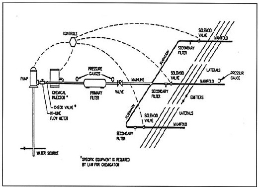
Figure V-2. Components of a typical drip irrigation system.
Some important trickle considerations and choices:
- Drip Tubing, Emitters, or Microsprinklers: Four types of drip tubing are shown in Figure V-3. Porous tubing such as “soaker hose” or “leaking pipe” has very poor uniformity and generally should not be used except in home gardens and landscape application. Drip strip tubing is commonly used on row crops due to its low cost (3 to 20 cents per foot) and includes such products as double walled tubing and drip tape (Figure V-3). These products deliver water from the center of the tubing to the outside using planned designs as shown in Figure V-4. Regulating tubes provide more uniform water application rates, especially for long laterals. Due to the wide variation in sites and designs, recommendations on the maximum lateral length cannot be made without manufacturer’s specifications. In most cases, however, row length in the 500 to 700 ft is suggested. Longer runs can be made but will require larger diameter more expensive drip tape. With proper filtration and maintenance (periodic flushing of lines, etc.), 15 or 16 mils wall tubing can have life spans ranging from 3 to 7 years, depending on product chosen. The less expensive 4 to 6 mils wall tubing generally can be used to produce 2 to 3 crops is the system is well managed. More expensive in-line barbed and thread type emitters are used primarily for permanent systems on high valued cash crops or as semiannual systems that are removed from the field and stored following the irrigation season. They tend to give better uniformity, and are less prone to clogging than strip tubing due to their larger orifices. Microsprinklers are used in situations where a large soil area needs to be wetted, such as in orchards and vineyards. They are very effective for protection against frost/freeze injury of tree crops, but generally are not used on row crops due to their high costs.
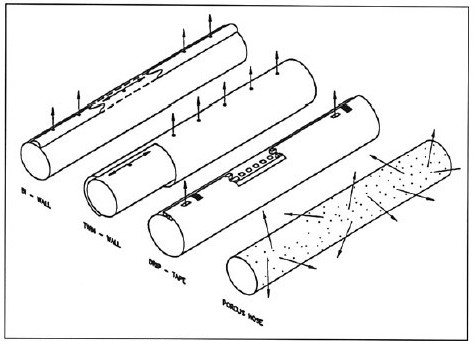
Figure V-3. Common types of drip strip tubing.
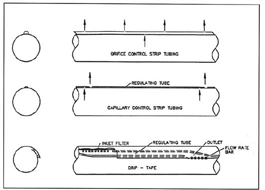
Figure V-4. Flow control design of common drip strip tubing.
- Buried or Surface: Buried lines tend to have less clogging problems, do not interfere with field operations and are not as often damaged by rodents. However, clogging problems are more difficult to see than with surface lines. In some areas, much damage to buried lines is caused by gophers and ants. Ants can be controlled by injection of insecticides where approved. Some manufacturers make special ant resistant tubing. Clogging of buried emitters by roots generally is not a problem. A typical tool for installing strip tubing is mounted on a tractor and is shown in Figure V-5. When burying, the emitter orifice should be facing upward toward the surface in order to reduce clogging problems and to allow soil particles to collect on the bottom of the tubing where they are easily flushed out. Most successful drip irrigators have found that surface applied tape creates serious management problems. The tape tends to ‘snake’ in the field with changes in temperature and high wind speed can blow tape off of the beds or out of the rows. Shallow burring alleviates these problems. The depth at which tape is buried depends upon the crop grow. However, tape placed 4 to 6 inches deep seems to work best in most cases for vegetable crops.
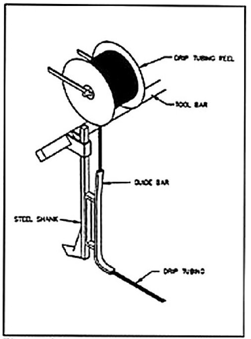
Figure V-5. Installation device commonly mounted on a tractor for burying drip strip tubing.
- Pressure or Nonpressure Compensating: Pressure compensating lines and emitters are used to maintain uniform discharges in spite of pressure changes caused by slope or high friction losses due to excessively long laterals. For many flat to small slope situations, adequate uniformity can be achieved with non-pressure compensating lines or emitters.
- Filters: One of the secrets to successful drip irrigation is proper filtration. Two types of filters are used: screen and media. Screen filters are the least expensive, and are used for relatively clean water sources such as wells or municipal supplies. Screen size needed depends on the size of the orifice of the emitter or drip line. Most drip strip tubing products require a 200 mesh screen. Media or sand filters are required where surface waters (streams, ponds, etc.) are used. Media filters are expensive, but may be equipped for automatic flushing, thus reducing maintenance. Manufacturers and irrigation dealers can supply the filtration requirements for particular products.
Although drip irrigation has been shown to increase yield, it is often difficult to justify their use based on yield increase alone due to the expense associated with these systems. Therefore, the decision to purchase a drip system should be based only on one or both of the following situations:
- Excessive Water Cost – The most effective means of reducing water cost is to reduce the volume of water needed to produce a crop. The increased water use efficiency of drip enables a significant reduction in the total volume required to satisfy crop needs. Additionally, less energy use is required to pump water with drip systems as compared to surface, sprinkler or pivot systems. As a result, the cost of water per unit of product produced is reduced.
- Limited Water Supply – To dealing with limited water supplies, vegetable producers are force to either reduce acreage or sacrifice crop yield. The reduced water volume required to produce a crop with drip affords the opportunity to optimally irrigate a crop or to expand irrigatable acreage.
Note: It must be remembered that plant water requirements cannot be reduce with any type of irrigation system, but rather, the volume of water needed to be delivered to a crop can be reduced.
As with the other types of irrigation systems, there are advantages and disadvantages to the use of drip irrigation.
Advantages of drip irrigation:
- Limited water sources can be used.
- Lower pressures are required to operate systems resulting in a reduction in energy for pumping.
- Precise water volume can be applied in the root zone (the area of use).
- Every plant in the field receives water nearly at the same moment.
- Other field operations such as harvesting and spraying can be done while irrigating.
- Reduction nutrient leaching, disease development, labor and operating costs are obtainable.
- Readily automated and well adapted to chemigation and fertigation.
Disadvantages of drip irrigation:
- High initial investment.
- Insects, rodents, and human damage occur readily to drip tape.
- High management.
- Cannot recover from a moisture deficit situation as readily as other systems.
- Used tape disposal.
Determining Irrigation Costs and Return on Investment
When deciding whether or not to irrigate, sound and complete economic analysis should be made. The first step is to estimate the potential increase in profits of irrigation over dry land or in going to a more efficient irrigation system. Your County Extension Agent can put you in touch with successful irrigators in your area; compare your yields to theirs. Next, estimate the cost of purchasing and operating the irrigation system. Your local irrigation dealer will provide cost estimates for different types of systems. Both the dealer and your local county extension agent can assist you in estimating the operating costs of different systems. Be sure to consider pumping, labor, and maintenance. These costs vary widely between systems. Table V-4 gives the annual maintenance and repair costs as a percent of initial costs for some irrigation system components.
Reference 1 discusses in detail irrigation costs analysis. Texas AgriLife Extension Publication L-2218 “Pumping Plant Efficiencies and Irrigation Costs” (Reference 6) is useful in evaluating pumping costs for different fuels and pumps. Texas AgriLife Extension also has available a low cost PC software package entitled “Irrigated vs. Dryland Crop Production” (AAU). This program is designed to take you step by step through the process of evaluating the costs and returns of irrigated versus dryland crop production including such factors as the cost of money and depreciation. Another program “Pumping Plant Efficiency and Fuel Costs” (AAR) is helpful in estimating seasonal pumping costs for different fuels. These packages can be purchased from Texas AgriLife Extension Software Distribution (979-845-3929). Most county extension offices have Texas AgriLife Extension software on their computers.
Table V-4. Annual Maintenance, Repairs, and Depreciation for Irrigation System Components
| Component | Depreciation (hours) | Period (year) | Annual Maintenance and Repair Percent of Initial Cost |
|---|---|---|---|
| Wells and Casings | – | 20 – 30 | 0.5 – 1.5 |
| Pumping Plant Structure | |||
| Pump, Vertical Turbine | – | 20 – 40 | 0.5 – 1.5 |
| Bowls | 16,000 – 20,000 | 8 – 10 | 5 – 7 |
| Column, etc. | 32,000 – 40,000 | 16 – 20 | 3 – 5 |
| Pump, Centrifugal | 32,000 – 50,000 | 16 – 25 | 3 – 5 |
| Power Transmission: Gear Head | 30,000 – 36,000 | 5 – 7 | |
| V-belt | 6,000 | 3 | 5 – 7 |
| Flat Belt, Rubber and Fabric | 10,000 | 5 | 5 – 7 |
| Flat Belt, Leather | 20,000 | 10 | 5 – 7 |
| Prime Movers: Electric Motor | 50,000 – 70,000 | 25 – 35 | 1.5 – 2.5 |
| Diesel Engine | 28,000 | 14 | 5 – 8 |
| Gasoline Engine: Air Cooled | 8,000 | 4 | 6 – 9 |
| Water Cooled Engine | 18,000 | 9 | 5 – 8 |
| Propane Engine | 28,000 | 14 | 4 – 7 |
| Open Farm Ditches (permanent) | 20 – 25 | 0.5 – 1.0 | |
| Concrete Structure | 20 – 40 | 0.5 – 1.0 | |
| Pipe: Asbestos, Cement, PVC (buried) | 40 | 0.25 – 0.75 | |
| Aluminum (surface) | 10 – 12 | 1.5 – 2.5 | |
| Steel, waterworks class, (buried) | 40 | 0.25 – 0.50 | |
| Steel, coated and lines, (buried) | 40 | 0.25 – 0.50 | |
| Steel, coated (buried) | 20 – 25 | 0.50 – 0.75 | |
| Steel, coated, (surface) | 10 – 12 | 1.5 – 2.5 | |
| Steel, galvanized (surface) | 15 | 1.0 – 2.0 | |
| Steel, coated and line (surface) | 20 – 25 | 1.0 – 2.0 | |
| Wood (buried) | 20 | 0.75 – 1.25 | |
| Aluminum, sprinkler use (surface) | 15 | 1.5 – 2.5 | |
| Reinforced Plastic Mortar (buried) | 40 | 0.25 – 0.50 | |
| Plastic (trickle, surface) | 10 | 1.5 – 2.5 | |
| Sprinkler Head | 8 | 5 – 8 | |
| Drip Emitters | 8 | 5 – 8 | |
| Drip Filters | 12 – 15 | 6 – 9 | |
| Land Grading | None | 1.5 – 2.5 | |
| Reservoirs | None | 2.0 – 2.0 | |
| Mechanical Move Sprinklers | 12 – 16 | 5 – 8 |
Source: G.T. Thompson, L.B. Spiess, and J.N. Krider, Farm Resources and System Selection, In Design and Operation of Farm Irrigation, Systems, 1980, M.E. Jensen (Ed.) ASAE Monograph 3, St. Joseph, MI, p. 45
Design Considerations
Design of an irrigation system should be done in a systematic and logical manner. The design process can be divided into 8 steps as listed below:
- Determine number of acres, types of crops and crop rotation plan.
- Estimate water supply required to meet crop needs. Be sure to adjust these rates for losses due to irrigation efficiencies (Table V-2) and other expected water losses. Also check with local growers, SCS personnel and irrigation dealers for water delivery rates used in your area.
- Determine if water supply is adequate. Generally, irrigation systems are designed to meet peak consumptive water use.
- Determine if water source is suitable. Have a water sample analyzed by the Texas AgriLife Extension Soil and Water Testing Lab.
- Select irrigation system.
- If using drip, select a filter system. For surface water sources, determine if settling ponds or screens are required.
- For sprinkler and drip systems, correctly size lateral, manifold and main pipelines. Improperly sized lines often result in excessive friction losses, increased pumping costs and poor water application uniformity. For surface systems, have length of runs and irrigation canals sized by SCS according to slope, soil type and water supply.
- Determine pump requirements include friction losses, operating pressure requirements and changes in elevation. Steps 6, 7, and 8 are very important, and often will determine the economics of operating the system. These should be done by a qualified irrigator or engineer.
The purchase, installation, operation and maintenance of irrigation systems are a major and significant capital expense. The long term economics of irrigation depends on the system being properly designed for your particular farm conditions.
Common problems that occur in improperly designed systems
- System capacity is too low to meet crop water needs.
- Too much or too little water is applied per application.
- System application rates exceed soil intake rates.
- Improperly sized mainlines and laterals result in excessive friction losses and a significant increase in pumping costs.
Selecting a Dealer
As in choosing any professional service, the selection of an irrigation dealer should be done carefully. Agricultural irrigation systems are exempt from regulation by the Texas Board of Irrigators (P.O. Box 12337, Capitol Station, Austin 78711, 512-463-7990). Thus, there is little recourse for the buyer of an improperly designed system. In selecting a dealer consider his qualifications, experience, reputation, knowledge, service record and references. Professional Agricultural Engineers do have the training for proper irrigation design and are on the staffs of several dealerships in Texas.
Irrigation Wells
When sizing irrigation well, you should consider the long term well costs and performance, not just the immediate or short term costs. Poorly designed or developed wells result in higher pumping costs and shorter pump life. Procedures exist that will ensure continuous sand free water supply, large yields, long pump and well life, and which will produce the most water for every dollar invested. These procedures are discussed in an unnumbered manuscript “Irrigation Well Design and Construction” by Dr. Don Reddell available through Ext. Ag. Engineering.
All well drillers in the State of Texas must be licensed by the Texas Water Well Drillers Board through the Texas Water Commission (TWC). In addition, the TWC has established minimum well standards and reporting requirements. For more information on the program or on the filing of complaints, contact the Texas Well Drillers Board at the TWC in Austin (512-371-6252).
The data in Table V-5 can be helpful in determining if irrigation well has the flow rate capacity to meet the intended crop acreage water demands. The number can be used to evaluate irrigation capacity with various irrigation well flow rates for daily, weekly and 30, to 100 day increment periods of pumping time. Water volumes are applicable for all irrigation systems and irrigatable acreage. They include application losses. Numbers represent 100% of the water but reflect irrigation capacity with highly efficient systems such as LEPA or drip (98%). Figure on 20% less for other conventional systems.
Table V-5. Required Flow Rate Capacity of Irrigation Wells inch/day
| gpm/acre | inch/week | Inches in Irrigation Days | |||||
|---|---|---|---|---|---|---|---|
| 30 | 45 | 60 | 80 | 100 | |||
| 1.5 | 0.55 | 0.08 | 2.4 | 3.8 | 4.8 | 6.4 | 8 |
| 2 | 0.75 | 0.11 | 3.2 | 4.8 | 6.4 | 8.5 | 10.6 |
| 2.5 | 0.93 | 0.13 | 4 | 6 | 8 | 10.6 | 13.3 |
| 3 | 1.1 | 0.16 | 4.8 | 7.2 | 9.5 | 12.7 | 15.9 |
| 3.5 | 1.3 | 0.18 | 5.6 | 8.3 | 11.1 | 14.8 | 18.6 |
| 4 | 1.5 | 0.21 | 6.4 | 9.5 | 12.7 | 17 | 21.2 |
| 4.5 | 1.67 | 0.24 | 7.2 | 10.7 | 14.3 | 19.1 | 23.9 |
| 5 | 1.85 | 0.27 | 8 | 11.9 | 15.9 | 21.2 | 26.5 |
| 5.5 | 2 | 0.29 | 8.7 | 13.1 | 17.5 | 23.3 | 29.2 |
| 6 | 2.25 | 0.32 | 9.5 | 14.3 | 19.1 | 25.4 | 31.8 |
| 6.5 | 2.41 | 0.34 | 10.3 | 15.5 | 20.7 | 27.5 | 34.4 |
| 7 | 2.6 | 0.37 | 11.1 | 16.7 | 22.6 | 29.7 | 37.1 |
To determine flow rates required, multiply the GPM per acre listed times the number of acres to irrigate to arrive at the flow rate needed to apply volume (inches) shown.
Example: 120 acres to be irrigated x 4 gpm/A = 480 gpm flow rate required to apply 1.5 inches of water per week
Pump Selection
Inefficient pumps and power units are major contributors to excessively high irrigation costs. To minimize fuel consumption and cost, pumping equipment must be carefully selected, properly maintained and replaced when necessary to maintain high efficiency. Efficient pumping plants, with their lower pumping cost combined with efficient application of carefully timed irrigations, can make the difference between profit and loss in irrigated crop production. For information on pumping plant selection and costs see Reference 1 and Texas AgriLife Extension publication L-2218 “Pumping Plant Efficiency and Irrigation Costs” (Reference 6). You should have a pumping plant efficiency test made at least every 5 to 8 years. Some electric utility companies and underground water conservation districts do pump efficiency testing at no charge.
Farm Water Delivery Systems
On-farm water delivery systems include lined and unlined canals and pipelines. As with other irrigation system components, you should carefully weigh the initial construction or purchase price against the long term costs of maintenance, pumping and/or the direct purchase costs of water. While earthen canals have low initial costs, the costs of the water lost to canal seepage may become significant over the canal’s lifetime. Transporting irrigation water through pipelines has proven to be the most trouble free and economical method.
Canals: Losses from irrigation canals result from both seepage into the surrounding soil and direct evaporation. Seepage losses may cause a water logged area or a salinity problem which is difficult to manage. Costs of water lost to seepage often will more than pay for lining materials or replacement pipelines. Unlined canals are sometimes acceptable in heavy clay soils which have low infiltration rates. Canals put in other soils will have low water delivery efficiencies. The SCS has developed guidelines for the design of canals.
Irrigation Pipelines: In sizing irrigation pipelines, the best size is not always the one with the lowest initial cost, but the size which minimizes the capital, pumping, maintenance and energy costs during the life of the system. Two factors are important: friction losses and water hammer; both of which are influenced by the relationship between flow rate (velocity) and pipe size.
Water hammer results from turbulent flow in the pipe. Water hammer may be caused by shock waves created by sudden increases or decreases in the velocity of the water or the lack of pressure relief valves. To prevent water hammer, a rule of thumb is to keep the water velocity at or below 5 feet/second. The exception is suction pipe lines for centrifugal pumps which should kept between 2 and 3 feet/second. Table V-6 lists the maximum flow rates recommended for different pipe sizes using the 5 feet/second rule.
Table V-6. Approximate Maximum Flow Rate in Different Pipe Sizes to keep Velocity at 5 ft/sec
| Pipe Diameter (inch) | Flow Rate (gpm) | Pipe Diameter (inch) | Flow Rate (gpm) |
|---|---|---|---|
| ½ | 6 | 4 | 200 |
| ¾ | 10 | 5 | 310 |
| 1 | 15 | 6 | 440 |
| 1¼ | 25 | 8 | 780 |
| 1½ | 35 | 10 | 1225 |
| 2 | 50 | 12 | 1760 |
| 3 | 110 | 16 | 3140 |
Excessive friction losses translate directly into higher power and thus, pumping costs. Select a pipe size appropriate for your flow rate. Smooth pipe has less friction loss, hence, lower operating cost than rough pipes. Plastic pipe, such as PVC, is the smoothest, followed by aluminum, steel and concrete, in that order. Table V-7 lists typical friction losses in commonly used pipe; it can be used for estimating operating costs for pipelines. More precise figures from manufacturers’ specifications should be used for design purposes.
Table V-7. Approximate Friction Losses in Feet of Head per 100 Feet of Pipe 2.5
| Pipe size | 4-inch | 6-inch | 8-inch | 10-inch | 12-inch | ||||||||||
|---|---|---|---|---|---|---|---|---|---|---|---|---|---|---|---|
| Steel | Alum. | PVC | Steel | Alum. | PVC | Steel | Alum. | PVC | Steel | Alum. | PVC | Steel | Alum. | PVC | |
| Flow Rate (gpm) | |||||||||||||||
| 100 | 1.2 | 0.9 | 0.6 | – | – | – | – | – | – | – | – | – | – | – | – |
| 150 | 1.8 | 1.2 | 0.3 | 0.2 | 0.2 | – | – | – | – | – | – | – | – | – | – |
| 200 | 4.3 | 3.0 | 2.1 | 0.6 | 0.4 | 0.3 | 0.1 | 0.1 | 0.1 | – | – | – | – | – | – |
| 250 | 6.7 | 4.8 | 3.2 | 0.9 | 0.6 | 0.4 | 0.2 | 0.1 | 0.1 | 0.1 | 0.1 | – | – | – | – |
| 300 | 9.5 | 6.2 | 4.3 | 1.3 | 0.8 | 0.6 | 0.3 | 0.2 | 0.1 | 0.1 | 0.1 | – | – | – | – |
| 400 | 16.0 | 10.6 | 7.2 | 2.2 | 1.5 | 1.0 | 0.5 | 0.3 | 0.2 | 0.2 | 0.1 | 0.1 | 0.1 | – | – |
| 500 | 24.1 | 17.1 | 11.4 | 3.4 | 2.4 | 1.6 | 0.8 | 0.6 | 0.4 | 0.3 | 0.2 | 0.1 | 0.1 | 0.1 | 0.1 |
| 750 | 51.1 | 36.3 | 24.1 | 7.1 | 5.0 | 3.4 | 1.8 | 1.3 | 0.8 | 0.6 | 0.4 | 0.3 | 0.2 | 0.1 | 0.1 |
| 1000 | 87.0 | 61.8 | 41.1 | 12.1 | 8.6 | 5.7 | 3.0 | 2.1 | 1.4 | 1.0 | 0.7 | 0.5 | 0.4 | 0.3 | 0.2 |
| 1250 | 131.4 | 93.3 | 62.1 | 18.3 | 3.0 | 8.6 | 4.5 | 3.2 | 2.1 | 1.5 | 1.1 | 0.7 | 0.6 | 0.4 | 0.3 |
| 1500 | 184.1 | 130.7 | 87.0 | 25.6 | 18.2 | 12.1 | 6.3 | 4.5 | 3.0 | 2.1 | 1.5 | 1.0 | 0.9 | 0.6 | 0.4 |
| 1750 | 244.9 | 173.9 | 115 | 34.1 | 24.2 | 16.1 | 8.4 | 6.0 | 4.0 | 2.8 | 2.0 | 1.3 | 1.2 | 0.9 | 0.6 |
| 2000 | 313.4 | 222.5 | 148.1 | 43.6 | 31.0 | 20.6 | 10.8 | 7.7 | 5.1 | 3.6 | 2.6 | 1.7 | 1.5 | 1.1 | 0.7 |
Note: Flow rates below horizontal line for each pipe size exceed the recommended 5 ft per second velocity.
Water Requirements, Irrigation Capacity and Scheduling Water Demands
The primary purposes of irrigation are to provide a soil environment for seed germination, seedling emergence and root development, and to supply sufficient water for plant growth and development. Soil moisture ideally is maintained in a range that permits absorption of water by the plant roots at a rate comparable to the plant’s transpiration. The amount of water a plant uses is affected by many factors, the most important of which are leaf area, stage of crop growth, climate and soil. Most plants also have critical periods during which significant reduction in yield and/or quality will occur if adequate water is not supplied. Critical periods for some vegetable crops are listed in Table 33 of the Appendix.
Unfortunately, little data is available on the water requirements of vegetables in Texas. The most extensive study of water requirements was conducted by the Texas Board of Water Engineers (Figure V-6). The average daily consumptive water use values of shallow and deep-rooted vegetables from this study are given in Tables 34 found in the Appendix for various regions of the State (Reference 7). Estimates of peak consumptive water use, based on climatic conditions, are presented Table 35 of the Appendix. Generally, irrigation systems are designed to supply the peak water demand of the plants. Peak water demand may be estimated from Tables 33 to 35. In some areas recommended rates may also be obtained from many local SCS offices and County Extension Agents.
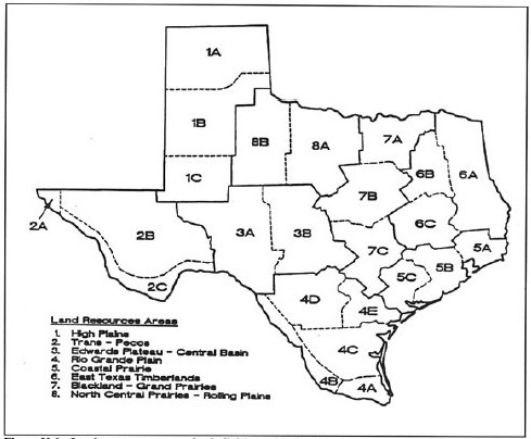
Figure V-6. Land resource areas and sub-divisions into irrigated areas.
Water Quality
To determine whether a source of water is suitable for irrigation, the water must be analyzed for:
- The total concentration of soluble salts
- The relative proportion of sodium to the other cations
- The bicarbonate concentration as related to the concentration of calcium and magnesium
- The concentration of toxic elements
In assessing water quality keep in mind that the water from the same source can vary in quality with time. Samples, therefore, should be tested at intervals throughout the year or during the potential irrigation period. The Soil and Water Testing Lab at Texas A&M University can do a complete analysis of irrigation water, and will provide a detailed computer printout on the interpretation of the analysis.
Salinity Hazard
Excess salt increases the osmotic pressure of the soil solution which can result in a physiological drought condition. That is, even though the field appears to have plenty of moisture, the plants wilt because the roots are unable to absorb the water. The total soluble salt content is often determined by measuring the electrical conductivity (EC) in millimhos per centimeter (mmhos/cm) at 25C or in micromhos per centimeter (µmhos/cm) (1 mmhos = 1000 µmhos) where µ is the Greek letter “mu”. In Table 36 of the Appendix the relative tolerance of some crops are listed by EC. Sometimes, the concentration of salt is measured directly and expressed in parts per million (ppm) or in the equivalent units of milligrams per liter (mg/l). Values for ppm, EC, and percent sodium are given in Table 37 of the Appendix.
Sodium Hazard
The sodium hazard of irrigation water usually is expressed as the sodium absorption ratio (SAR). SAR is the relationship between sodium, calcium and magnesium. It is used to evaluate the effects of irrigation water on the soil. Continuous use of water with high SAR leads to a breakdown in the physical structure of the soil due to the absorption of sodium onto the soil particles and the resulting dispersion of the clay particles. The soil then becomes hard and compact when dry and increasingly impervious to water penetration. Fine textured soils, especially those high in clay are especially subject to this action. Calcium and magnesium, if present in large enough quantities, will counter the effects of the sodium and help maintain good soil properties. Appendix, Table 39 gives classification of sodium hazard based on SAR. Gypsum can be economically on some soils used to maintain the soil, even with high SAR.
Sometimes the soluble sodium per cent (SSP) is used to evaluate sodium hazard. SSP is defined as the ration of sodium in epm (equivalents per million) to the total cation epm multiplied by 100. Water with a SSP greater than 60 per cent may result in sodium accumulations that will cause a breakdown in the soil’s physical properties.
Toxic Elements
The three major toxic elements of concern are; chlorides (Cl), sulfates SO4 and boron. Good information is available on the toxicity of boron on many crops (Appendix, Table 36). General permissible levels of Cl and SO4 are given in Table 37 of the Appendix. Contact Texas AgriLife Extension Soil and Water Testing Lab (979-845-4816) for more information.
Salinity Management Techniques
The best management approach depends on many factors, including the nature and severity of the salinity problem, soil type and water intake rate. In many situations, water is applied in excess of the amounts used by the plants in order to keep the salts in solution and flush them below the root zone. The amount of water needed is referred to as the leaching fraction. In some areas natural rainfall over winter months provides adequate leaching. Table 38 in the Appendix, gives the number of one-inch irrigations possible with various salinity levels between leaching rains.
Salinity control procedures that require relatively minor changes in management are more frequent irrigations, selection of more salt tolerant crops, additional leaching, preplant irrigation, bed forming and seed placement. Alternatives that require significant changes in management are changing the irrigation method, altering the water supply, land grading, modifying the soil profile and installing artificial drainage. For more information see Reference 14. The County Extension Agent also can put you in touch with Extension Agricultural Engineers and Soil Chemists for additional information and assistance.
Irrigation Scheduling
Irrigation scheduling is the process of determining when to irrigate and how much water to apply per irrigation. Proper scheduling is essential for the efficient use of water, energy and other production inputs such as fertilizer. It allows irrigations to be coordinated with other farming activities including cultivation and chemical applications. Among the benefits of proper irrigation scheduling are improved crop yield and/or quality, conservation of water and energy, and, lower production costs.
Deficit irrigation is the practice of partially supplying the irrigation requirements of crops. Deficit irrigation with planned soil moisture storage is often used to reduce the needed irrigation amounts during peak consumptive use periods by taking advantage of the natural ability of soils to hold water. The concept is simple: excess water is applied during the early season and stored in the soil profile for later use. Using the planned soil moisture storage is an excellent strategy for situations where the water supply or the irrigation system is insufficient to meet peak water demands of crops. Soil moisture monitoring is recommended in order to prevent the application of too much water which would move below the root zone and become unavailable to the plants.
Deficit irrigation also is used in situations where reducing water applications causes production costs to decrease faster than revenues decline as a result of reduced yield and quality. Deficit irrigation is often unintentionally used when the irrigation system or water supply is inadequate to supply the plant’s water requirements. Many vegetable crops are very sensitive to drought conditions, and will only produce adequately with proper amounts of water. In cases of limited water supply, be sure to irrigate during the most critical growth period (Appendix, Table 33).
Methods used to determine when to irrigate:
- Plant indicators
- Water budget techniques
- Soil moisture measurement
Plant indicators involve monitoring the plant’s appearance for signs of water stress. Contact Extension Horticulture for more information. The water budget techniques normally use equations to predict irrigation requirements based on climatic and site factors. These methods are discussed in References 2 and 9.
Directly monitoring the moisture content of the soil in the root zone takes much of the guess work out of irrigation scheduling. Usually, either tensiometers or gypsum blocks (sometimes called porous or electrical resistance blocks) are used to measure the moisture content of the soil. Both have dial or digital readings which can be related to the water pressure in the soil. Table V-8 shows a suggested correlation between tensiometer readings and soil moisture levels for vegetable production. Gypsum block meters often have a scale of 0 to 100. Check the manufacturer’s literature for the correct interpretation. Gypsum blocks tend to be more trouble free, and are often more economical for large acreage. Details on soil moisture monitoring are in Texas AgriLife Extension Publication B-1610 “Soil Moisture Monitoring” (Reference 10).
Table V-8. Interpretation of Tensiometer Readings for Vegetables
| Dial Reading in Centibars | Interpretation | |
|---|---|---|
| Nearly saturated | 0 | Nearly saturated soil often occurs for a day or two following irrigation. Danger of water-logged soils, a high water table, poor soil aeration, or the tensiometer may have broken tension if readings persist. |
| Field capacity | 10 | Field capacity. Irrigations discontinued at field capacity to prevent waste by deep percolation and leaching of nutrients below the root zone. |
| Irrigation range | 20 | Usual range for starting irrigations. Most of the available soil moisture is used up in sandy loam soils. For clay loams, only one or two days of soil moisture remain. |
| Dry | 3080 | This is the stress range for most vegetable crops. Top range of accuracy of tensiometer. Readings above this are possible but many tensiometers will break tension between 80 to 85 centibars. |
The amount of water that should be applied during irrigation depends on the current moisture content in the root zone and the amount of water it takes to “fill” the root zone (or bring it up to field capacity.) These concepts are discussed in Texas AgriLife Extension Publication “Soil Moisture Management” (Reference 11.) Keep in mind that in addition to the crop consumptive use, the total irrigation amount must include enough water to make up for losses due to irrigation efficiency, deep percolation, wind drift, etc., as illustrated in Figure V-7. It is important to know the depth of the active root zone in order to make efficient use of the irrigation water. Field observations are best. Table 14 of the Appendix, gives approximate rooting depths of mature vegetable crops in a deep, well drained soil. The soil infiltration rate plays a big role in determining how long the irrigation run time should be as well as the system delivery rate. Table V-9 list the maximum water infiltration rate of various soil types.
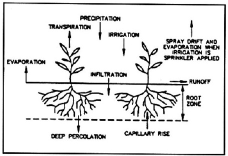
Figure V-7. Sources and losses of soil moisture.
Table V-9. Maximum Water Infiltration Rate in Various Soil Types
| Soil Type | Infiltration Rate (inch/hr)* |
|---|---|
| Sand | 2 |
| Loamy sand | 1.8 |
| Sandy loam | 1.5 |
| Loam | 1 |
| Silt and clay loam | 0.5 |
| Clay | 0.2 |
* Assumes a full crop cover. Bare soil rate is ½ of full crop cover
Drip Clogging Control
The biggest potential problem facing the operator of a drip irrigation system is emitter clogging. Because the water passages in most emitters are very small, they easily become clogged by minerals or organic matter. Clogging can reduce output and cause poor water distribution which may cause stress and damage to plants. Contaminants are often present in the irrigation water, such as soil particles, living or dead organic materials and scale from rusty pipes. Contaminants may also enter the system during the installation phase. These include insects, Teflon tape, PVC pipe shavings and soil particles which should be flushed out of the lines before closing drip lines or attaching sprinkler heads.
Contaminants also may grow, aggregate or precipitate in water as it stands in the lines or evaporates from emitters or orifices between irrigations. Iron oxide, manganese dioxide, calcium carbonate, algae and bacterial slimes can form in drip systems under certain circumstances.
The solution to clogging must be based on the nature of the particular problem. The following procedures, taken from The Pecan Profitability Handbook (Reference 12) are helpful in correcting clogging problems in drip irrigation systems.
Mineral Deposits
Calcium and magnesium: Minerals cannot be removed by filtration and some, particularly Ca, Mg and iron, often form precipitates in field line and emitters. If the precipitates are not removed, serious emitter plugging will occur.
Periodic drip system acidification will aid in removing these precipitates. Technical grade sulfuric acid is relatively inexpensive and thus, is probably the most practical material. Phosphoric acid and hydrochloric (muriatic) acid also can be used.
Several guidelines on acidification are listed below:
- How often should acid be injected? When there is more than 10% flow reduction from mineral buildup in emitters. With regular use in an average system this will be about twice per year.
- How much acid should be injected? Enough to drop the pH of water in the field lines to about 3.5. This will usually require 1 part acid per 2,000 parts water.
- During what part of the cycle should acid be injected? Near the end. Allow enough time for all the lines to be acidified before the system is turned off. Leave the acidified water in the lines for at least an hour or overnight before turning the system back on to flush the lines.
- Where acid should be injected? Downstream from the filter.
- Where acid can be purchased? Thompson Hayward Chemical Company outlets in Houston, Dallas, San Antonio, Odessa and Beaumont sell sulfuric acid, primarily in 200-pound carbons. Check local chemical dealers for other sources. Muriatic acid can usually be purchased from swimming pool companies and various lumber yards.
Iron: Control of stoppage caused by iron deposits can be more difficult than simple acid injection if iron levels in the water are high. Where iron problems are suspected, water samples need to be analyzed to determine the iron level. General stoppage control methods depend on the iron level.
Iron less than 7 to 8 ppm: Use acidification as discussed for calcium and magnesium. Ideally, inject acid at least every two weeks.
Iron 8 to 12 ppm: Use gaseous chlorination. This will require a sand filter to catch the precipitate. This cannot be done inexpensively; chlorine injectors and sand filters are relatively costly. Chlorine gas is dangerous and must be handled with extreme care.
Iron more than 13 ppm: Use a settling basin (pond) where expose to air can oxidize and precipitate iron. At least 15 to 30 minutes of air exposure should be allowed for iron to oxidize and precipitate.
Algae and Bacteria
Algae, and in some cases, bacteria can cause severe emitter clogging. Algae can be particularly severe when surface water is used in drip systems. Chlorination can effectively stop the growth of algae and bacteria in drip systems.
Guidelines on chlorination are listed below. Additional guidelines for chemical treatment are given in Table V-10.
- What sources of chlorine can be used? Liquid bleach sodium hypochlorite at 5.25% is most common. Sodium hypochlorite Solutions with 10.5 and 15.0% also are available. Dry granular chlorine should not be used because of precipitate problems. In large systems (greater than 400 ppm) to save money, chlorine gas is often used. Chlorine gas is dangerous.
- How often should chlorine be injected? Every time the system is operated if surface water is used. Well water does not normally require chlorination for algae, but bacteria can sometimes be a problem. If there are few problems, with experience, the frequency may be reduced.
- How much chlorine should be injected? Enough to leave at least 1.25 ppm free residual chlorine in the drip lines. To achieve 1 to 2 ppm free residual chlorine in the lines will normally require injection of 10 to 12 ppm chlorine but this varies according to the amount of organic material and pH of the water. To test for free residual chlorine, a DPD chlorine testing kit is needed. These are inexpensive and are manufactured by Hatch Company, Ames, Iowa.
- During what part of the cycle should the chlorine be injected? Near the end. Allow enough time for all the lines to be chlorinated before the system is turned off.
- Where chlorine should be injected? Preferably upstream from the filter, since chlorine will help control algae in the filter.
Table V-10. Recommended Chemical Treatments for Selected Conditions
| Water Quality | Suggested Treatment |
|---|---|
| Ca > 50 ppmMg > 50 ppm | Hard water, caused by high ppm concentrations of Ca or Mg, can reduce flow rates by the buildup of scales on pipe walls and emitter orifices. Periodic injection of an HCl solution may be required throughout the season. Lower concentrations of Ca and Mg may require HCl treatment every few years. |
| Fe > 0.5 ppmS > 0.5 ppm | Iron and sulfur, as well as other metal contaminants, provide an environment in water that is conducive to bacterial activity. The by-products of the bacteria in combination with the fine (less than 100-micron) suspended solids can cause system plugging. Bacterial activity can be controlled by chlorine injection and line flushing on a regular basis throughout the irrigation season. Bacterial activity is prevalent in Fe and S concentrations S over 0.5 ppm, but may also occur at lower concentrations. |
Source: British Columbia Ministry of Agriculture, Water Treatment Guidelines for Trickle Irrigation, Engineering Reference Information R512.000, 1982. 2 pp.
Chemigation
Chemigation is the application of fertilizer, herbicides, insecticides, fungicides and other chemicals through irrigation systems. Recent advances in chemigation equipment and know how have given growers a method of improving the effectiveness of chemicals while reducing the amounts applied. The U.S. Environmental Protection Agency has developed regulations on types of chemigation equipment allowed with the aim of preventing accidents, thereby, protecting both the grower and the environment. These are covered in “Chemigation Workbook” (Reference 13).
Irrigating with Effluent
The Texas Water Commission has developed regulations on the use of municipal effluent water for irrigation. These regulations prohibit spray irrigation of effluent water on food crops. Also, fodder, fiber and seed crops may not be harvested within 30 days of application of reclaimed water. For more information, contact the TWC in Austin (512-463-8412).
Monitoring System Performance
The well designed irrigation system will have built-in diagnostic tools which allow the operator to monitor the performance of the system and to detect possible problems in early stages. The most important devices are flow meters and pressure gauges. System flow meters should be installed on the main supply lines, and should provide readings of both instantaneous and cumulative flow. These meters should be read regularly and the readings kept in a log book. Variations in the system flow rate may indicate that something in the system is amiss. Some possible causes of changes in irrigation system flow are given in Table V-11.
Table V-11. Possible Causes of Changes in Irrigation System Flow
| Increased Flow | Improperly adjusted gates, valves, checks Pipeline leaks and breaks Pressure downstream of pressure regulators is too high Worn or oversize sprinkler nozzles, emission devices, etc. System on too long (as indicated by higher than expected volumes of flow) |
|---|---|
| Decreased flow | Improperly adjusted gates, valves, checks Clogged sprinklers, emission devices, screens, filters, etc. Pressure downstream of pressure regulators too low. Existence of entrapped air in the system System not on long enough (as indicated by lower than expected volumes of flow) |
The system should have sufficient pressure testing points, so that an overall check of the system pressures can be made. Widely differing pressures in different sections of the system may indicate that some blockage, leaking or other problem has arisen in some section of the system. Pressure checks should be regularly made and the pressures recorded. Center pivots should have a pressure gauge at the end of the system (instead of only at the pivot point).
Annual maintenance and repairs should be incorporated into the normally expected operation expenses of the system. Worn components should be replaced as needed. Generalized depreciation and annual maintenance and repairs are listed in Table V-4. When possible, use data provided by manufacturers.
References
- Turner, J. H. and C. L. Anderson. 1980. Planning for an Irrigation System. Published by American Association for Vocational Instructional Materials, Athens, GA. 120 pp.
- James, L. G. 1993. Principles of Farm Irrigation System Design. Published by Krieger Publishing Company. 560 pp.
- Henggeler, J. C., J. M. Sweeten and C. W. Keese. 1986. Surge flow irrigation. L-2220, Texas AgriLife Extension
- Henggeler, J. C. 1986. Irrigation Systems for Forage Crops. B-1611, Texas AgriLife Extension.
- New, L. L. 1986. Center Pivot Irrigation Systems. B-2219, Texas AgriLife Extension.
- New, L. L. 1986. Pumping Plant Efficiency and Irrigation Costs. L-2218, Texas AgriLife Extension.
- McDaniels, L. L. 1962. Consumptive use of water by major crops in Texas. Bulletin 6019, Texas Board of Water Engineers.
- Longenecker, D. E., and P. J. Lyerly. 1974. Control of Soluble Salts in Farming and Gardening. B-876. Texas AgriLife Extension.
- Jensen, M. E. 1982. Design and Operation of Farm Irrigation Systems. American Society of Agricultural Engineers, St. Joseph, MI. 829 pp.
- Sweeten, J. M. and J.C Henggeler. 1988. Soil Moisture Monitoring. B-1610, Texas AgriLife Extension.
- Fipps, G. 1990. Soil Moisture Management. B-1970, Texas AgriLife Extension.
- McEachern, G. R. and L. A. Stein. 1990. Texas Pecan Profitability Handbook. Texas AgriLife Publication.
- New, L. L., A. Knutson, B. W. Bean, W. P. Morrison, C. D. Patrick, M. G. Hickey, H. W. Kaufman, T. Lee, S. H. Amosson, D. McWilliams, G. Fipps, and J. Sweeten. Chemigation Workbook. B-1652, Texas AgriLife Extension.
- Fipps, G. 1996. Managing Irrigation Water Salinity in the Lower Rio Grande Valley. B-1667, Texas AgriLife Extension.
- Hanson, B., L. Schwankl, S. Grattan, and T. Prichard. 1996. Drip Irrigation for Row Crops. University of California Irrigation Program. UC, Davis. Water Management Series. Publication #93-05.